Excel Dmax function

DMAX

What Does It Do ?

This function examines a list of information and produces the largest value from a specified column.

Syntax

=DMAX(DatabaseRange,FieldName,CriteriaRange)

The DatabaseRange is the entire list of information you need to examine, including the field names at the top of the columns.

The FieldName is the name or cell, of the values to pick the Max from, such as "Value Of Stock" or I3.

The CriteriaRange is made up of two types of information.

The first set of information is the name, or names, of the Fields(s) to be used as the basis for selecting the records, such as the category Brand or Wattage.

The second set of information is the actual record, or records, which are to be selected, such as Horizon as a brand name, or 100 as the wattage.

Formatting

No special formatting is needed.

Examples

The largest Value Of Stock of a particular Product of a particular Brand.

Use Excel's SUMPRODUCT To Summarize Worksheet Data

SUMPRODUCT

What Does It Do ?

This function uses at least two columns of values. The values in the first column are multipled with the corresponding value in the second column. The total of all the values is the result of the calculation.

Syntax

=SUMPRODUCT(Range1, Range, Range3 through to Range30)

Formatting

No special formatting is needed.

Example

The following table was used by a drinks merchant to keep track of stock.

The merchant needed to know the total purchase value of the stock, and the potential value of the stock when it is sold, takinging into account the markup percentage.

The =SUMPRODUCT() function in Excel is used to multiply the Cases In Stock with the Case Price to calculate what the merchant spent in buying the stock.

The =SUMPRODUCT() function in Excel is used to multiply the Cases In Stock with the Bottles In Case and the Bottle Setting Price, to calculate the potential value of the stock if it is all sold.

How to edit a cell of text in Excel ?

What Does It Do ?

This function replaces a specified piece of text with a different piece of text. It can either replace all occurrences of the text, or a specific instance. The function is case sensitive.

Syntax

=SUBSTITUTE(OriginalText,TextToRemove,TextToInsert,InstanceToUse) The InstanceToUse is optional, if it is omitted all instances will be substituted.

Formatting

No special formatting is needed.

Note

To cope with upper or lower case in the substitution you can use other text functions such as =UPPER(), =LOWER() or =PROPER() to ensure that the substitution will take place.

Table 1 shows how differing text cases alter the result of the substitution.

VLOOKUP

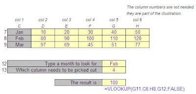
What Does It Do ?

This function scans down the row headings at the side of a table to find a specified item. When the item is found, it then scans across to pick a cell entry.

Syntax

=VLOOKUP(ItemToFind,RangeToLookIn,ColumnToPickFrom,SortedOrUnsorted)

The ItemToFind is a single item specified by the user.

The RangeToLookIn is the range of data with the row headings at the left hand side.

The ColumnToPickFrom is how far across the table the function should look to pick from.

The Sorted/Unsorted is whether the column headings are sorted. TRUE for yes, FALSE for no.

Formatting

No special formatting is needed.

Example 1

This table is used to find a value based on a specified name and month.

The =VLOOKUP() is used to scan down to find the name.

The problem arises when we need to scan across to find the month column.

To solve the problem the =MATCH() function is used.

The =MATCH() looks through the list of names to find the month we require. It then calculates the position of the month in the list. Unfortunately, because the list of months is not as wide as the lookup range, the =MATCH() number is 1 less than we require, so and extra 1 is added to compensate.

The =VLOOKUP() now uses this =MATCH() number to look across the columns and picks out the correct cell entry.

The =VLOOKUP() uses FALSE at the end of the function to indicate to Excel that the row headings are not sorted.

Example 2

This example shows how the =VLOOKUP() is used to pick the cost of a spare part for different makes of cars.

The =VLOOKUP() scans down row headings in column F for the spare part entered in column C. When the make is found, the =VLOOKUP() then scans across to find the price, using the result of the =MATCH() function to find the position of the make of car.

The functions use the absolute ranges indicated by the dollar symbol . This ensures that when the formula is copied to more cells, the ranges for =VLOOKUP() and =MATCH() do not change.

Example 3

In the following example a builders merchant is offering discount on large orders.

The Unit Cost Table holds the cost of 1 unit of Brick, Wood and Glass.

The Discount Table holds the various discounts for different quantities of each product.

The Orders Table is used to enter the orders and calculate the Total.

All the calculations take place in the Orders Table.

The name of the Item is typed in column C of the Orders Table.

The Unit Cost of the item is then looked up in the Unit Cost Table.

The FALSE option has been used at the end of the function to indicate that the product names down the side of the Unit Cost Table are not sorted.

Using the FALSE option forces the function to search for an exact match. If a match is not

found, the function will produce an error.

=VLOOKUP(C126,C114:D116,2,FALSE)

The discount is then looked up in the Discount Table

If the Quantity Ordered matches a value at the side of the Discount Table the =VLOOKUP will look across to find the correct discount.

The TRUE option has been used at the end of the function to indicate that the values

down the side of the Discount Table are sorted.

Using TRUE will allow the function to make an approximate match. If the Quantity Ordered does not match a value at the side of the Discount Table, the next lowest value is used.

Trying to match an order of 125 will drop down to 100, and the discount from the 100 row is

used.

=VLOOKUP(D126,F114:I116,MATCH(C126,G113:I113,0)+1,TRUE)

Formula for :

Unit Cost =VLOOKUP(C126,C114:D116,2,FALSE) Discount

=VLOOKUP(D126,F114:I116,MATCH(C126,G113:I113,0)+1,TRUE)

Total =(D126*E126)-(D126*E126*F126)