How to edit a cell of text in Excel ?

What Does It Do ?

This function replaces a specified piece of text with a different piece of text. It can either replace all occurrences of the text, or a specific instance. The function is case sensitive.

Syntax

=SUBSTITUTE(OriginalText,TextToRemove,TextToInsert,InstanceToUse) The InstanceToUse is optional, if it is omitted all instances will be substituted.

Formatting

No special formatting is needed.

Note

To cope with upper or lower case in the substitution you can use other text functions such as =UPPER(), =LOWER() or =PROPER() to ensure that the substitution will take place.

Table 1 shows how differing text cases alter the result of the substitution.

In Excel Find number of combinations for fixed number of items.

COMBIN

What Does It Do ?

This function calculates the highest number of combinations available based upon a fixed number of items. The internal order of the combination does not matter, so AB is the same as BA.

Syntax

=COMBIN(HowManyItems,GroupSize)

Formatting

No special formatting is required.

Example 1

This example calculates the possible number of pairs of letters available from the four characters ABCD.

Example 2

A decorator is asked to design a colour scheme for a new office. The decorator is given five colours to work with, but can only use three in any scheme. How many colours schemes can be created ?

How to deal with Excel Formula Errors - using ISERROR & IFERROR

ISERROR

What Does It Do ?

This function tests a cell or calculation to determine whether an error has been generated. It will show TRUE for any type of error and FALSE if no error is found.

Syntax

=ISERROR(CellToTest) The CellToTest can be a cell reference or a formula.

Formatting

No special formatting is needed.

Example

The following tables was used to calculate the difference between two dates.

Table 1 shows an error due to the fact that the first entry was entered using an inappropriate date format.

Table 2 shows how the =ISERROR() function has been used to trap the error and inform the user that there has been an error in the data entry.

IFERROR

Syntax

IFERROR(value,value_if_error)

Value_if_error is the value to return if the formula evaluates to an error. The following error types are evaluated: #N/A, #VALUE!, #REF!, #DIV/0!, #NUM!, #NAME?, or #NULL!.

Remarks

• If value or value_if_error is an empty cell, IFERROR treats it as an empty string value ("").
• If value is an array formula, IFERROR returns an array of results for each cell in the range specified in value. See the second example below.

How to use if statements in Excel

What Does It Do?

This function tests a condition.

If the condition is met it is considered to be TRUE.

If the condition is not met it is considered as FALSE. Depending upon the result, one of two actions will be carried out.

Syntax

=IF(Condition,ActionIfTrue,ActionIfFalse)

The Condition is usually a test of two cells, such as A1=A2.

The ActionIfTrue and ActionIfFalse can be numbers, text or calculations.

Formatting

No special formatting is required.

Example 1

The following table shows the Sales figures and Targets for sales reps.

Each has their own target which they must reach.

The =IF() function is used to compare the Sales with the Target.

If the Sales are greater than or equal to the Target the result of Achieved is shown.

If the Sales do not reach the target the result of Not Achieved is shown.

Note that the text used in the =IF() function needs to be placed in double quotes "Achieved".

Example 2

The following table is similar to that in Example 1. This time the Commission to be paid to the sales rep is calculated. If the Sales are greater than or equal to the Target, the Commission is 10% of Sales. If the Sales do not reach Target, the Commission is only 5% of Sales.

Example 3

This example uses the =AND() within the =IF() function.

A builders merchant gives 10% discount on certain product lines.

The discount is only given on products which are on Special Offer, when the Order Value is £1000 or above.

The =AND() function is used with the =IF() to check that the product is on offer and that the value of the order is above £1000.

Formula for counting Blank in Excel

What Does It Do ?

This function counts the number of blank cells in a range.

Syntax

=COUNTBLANK(RangeToTest)

Formatting

No special formatting is needed.

Example

The following table was used by a company which was balloting its workers on whether the company should have a no smoking policy. Each of the departments in the various factories were questioned. The response to the question could be Y or N. As the results of the vote were collated they were entered in to the table.

The =COUNTBLANK() function has been used to calculate the number of departments which have no yet registered a vote.

VLOOKUP

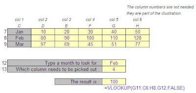
What Does It Do ?

This function scans down the row headings at the side of a table to find a specified item. When the item is found, it then scans across to pick a cell entry.

Syntax

=VLOOKUP(ItemToFind,RangeToLookIn,ColumnToPickFrom,SortedOrUnsorted)

The ItemToFind is a single item specified by the user.

The RangeToLookIn is the range of data with the row headings at the left hand side.

The ColumnToPickFrom is how far across the table the function should look to pick from.

The Sorted/Unsorted is whether the column headings are sorted. TRUE for yes, FALSE for no.

Formatting

No special formatting is needed.

Example 1

This table is used to find a value based on a specified name and month.

The =VLOOKUP() is used to scan down to find the name.

The problem arises when we need to scan across to find the month column.

To solve the problem the =MATCH() function is used.

The =MATCH() looks through the list of names to find the month we require. It then calculates the position of the month in the list. Unfortunately, because the list of months is not as wide as the lookup range, the =MATCH() number is 1 less than we require, so and extra 1 is added to compensate.

The =VLOOKUP() now uses this =MATCH() number to look across the columns and picks out the correct cell entry.

The =VLOOKUP() uses FALSE at the end of the function to indicate to Excel that the row headings are not sorted.

Example 2

This example shows how the =VLOOKUP() is used to pick the cost of a spare part for different makes of cars.

The =VLOOKUP() scans down row headings in column F for the spare part entered in column C. When the make is found, the =VLOOKUP() then scans across to find the price, using the result of the =MATCH() function to find the position of the make of car.

The functions use the absolute ranges indicated by the dollar symbol . This ensures that when the formula is copied to more cells, the ranges for =VLOOKUP() and =MATCH() do not change.

Example 3

In the following example a builders merchant is offering discount on large orders.

The Unit Cost Table holds the cost of 1 unit of Brick, Wood and Glass.

The Discount Table holds the various discounts for different quantities of each product.

The Orders Table is used to enter the orders and calculate the Total.

All the calculations take place in the Orders Table.

The name of the Item is typed in column C of the Orders Table.

The Unit Cost of the item is then looked up in the Unit Cost Table.

The FALSE option has been used at the end of the function to indicate that the product names down the side of the Unit Cost Table are not sorted.

Using the FALSE option forces the function to search for an exact match. If a match is not

found, the function will produce an error.

=VLOOKUP(C126,C114:D116,2,FALSE)

The discount is then looked up in the Discount Table

If the Quantity Ordered matches a value at the side of the Discount Table the =VLOOKUP will look across to find the correct discount.

The TRUE option has been used at the end of the function to indicate that the values

down the side of the Discount Table are sorted.

Using TRUE will allow the function to make an approximate match. If the Quantity Ordered does not match a value at the side of the Discount Table, the next lowest value is used.

Trying to match an order of 125 will drop down to 100, and the discount from the 100 row is

used.

=VLOOKUP(D126,F114:I116,MATCH(C126,G113:I113,0)+1,TRUE)

Formula for :

Unit Cost =VLOOKUP(C126,C114:D116,2,FALSE) Discount

=VLOOKUP(D126,F114:I116,MATCH(C126,G113:I113,0)+1,TRUE)

Total =(D126*E126)-(D126*E126*F126)