Create a Drop Down List in Excel

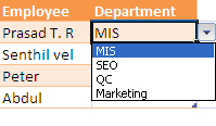
To make data entry easier in Excel, or to limit entries to certain items that you define, you can create a drop-down list of valid entries that is compiled from cells elsewhere on the worksheet. When you create a drop-down list for a cell, it displays an arrow next to that cell. To enter information in that cell, click the arrow, and then click the entry that you want.


We can create drop-down list by using " Data Validation" in Data menu.

1. To create a list of valid entries for the drop-down list, type the entries in a single column or row without blank cells. For example:

2.Then select the cell where you want to apply drop-down list.

3. To open Data validation window Click "Data Validation" option in Data menu

4. Choose "List"  in drop-down menu and choose the source.

It will through the Error message if we do manual entry. We can also customise the Error message.

Error Window

 

Select "Error Alert" Tab in Data Validation window. 

After enter the error message click OK. after that you will get follow error message.

To delete a drop down list, select the cell with the list. Click the Data menu, and then click Validation. In the Data Validation dialog box, click the Settings tab, and then click Clear All.

The maximum number of entries that you can have in a drop-down list is 32,767.

Microsoft Excel DGET formula

DGET

We can use DGET function when we have multiple criteria, we can use this as a alternative function of VLOOKUP function.

    How many boxes of a particular item do we have in stock?

     What Does It Do ? 

 This function examines a list of information and produces one result. If more than one record matches the criteria the error #NUM is shown. If no records match the criteria the error #VALUE is shown.

     

    Syntax

=DGET(DatabaseRange,FieldName,CriteriaRange) 

 The DatabaseRange is the entire list of information you need to examine, including the field names at the top of the columns. 

 The FieldName is the name, or cell, of the values to Get, such as "Value Of Stock" or I3. 

 The CriteriaRange is made up of two types of information.

 The first set of information is the name, or names, of the Fields(s) to be used as the basis    for selecting the records, such as the category Brand or Wattage.    

The second set of information is the actual record which needs to be selected, such     as Horizon as a brand name, or 100 as the wattage. 

Formatting
 No special formatting is needed.

Example 1
 This example extracts information from just one record.

 How many boxes of a particular item do we have in stock?

Example 2 

 This example extracts information from multiple records and therefore shows the #NUM error. 

 How many boxes of a particular item do we have in stock?  

Example 3 

 This example extracts information from no records and therefore shows the #VALUE error. 

 How many boxes of a particular item do we have in stock? 

Example 4 

 This example uses the =IF() function to display a message when an error occurs. How many boxes of a particular item do we have in stock?  

 =IF(ISERR(F88),CHOOSE(ERROR.TYPE(F88)/3,"No such product.","Duplicates products found."),"One product found.")

  

How to use Ms Excel SUM and the =OFFSET function

    SUM and the =OFFSET function


       Sometimes it is necessary to base a calculation on a set of cells in different locations. An example would be when a total is required from certain months of the year, such as the last 3 months in relation to the current date.

One solution would be to retype the calculation each time new data is entered, but this would be time consuming and open to human error.

     A better way is to indicate the start and end point of the range to be calculated by using the =OFFSET() function.

The =OFFSET() picks out a cell a certain number of cells away from another cell. By giving the =OFFSET() the address of the first cell in the range which needs to be totalled, we can then indicate how far away the end cell should be and the =OFFSET() will give us the address of cell which will be the end of the range to be totalled.

The =OFFSET() needs to know three things; 1. A cell address to use as the fixed point from where it should base the offset. 2. How many rows it should look up or down from the starting point. 3. How many columns it should look left or right from the starting point.

                                  =SUM(E24:OFFSET(E24,0,0))
This example uses E24 as the starting point and offsets no rows or columns which results in the range being summed as E24:E24.

                                    =SUM(E29:OFFSET(E29,0,1))
This example uses E29 as the starting point and offsets 1 col to pick out cell F29 resulting in a the range E29:F29 being summed.

                                    =SUM(E34:OFFSET(E34,0,2))
This example uses E34 as the starting point and offsets 2 cols to pick out
cell G34 resulting in a the range E34:G34 being summed.




Using =OFFSET() Twice In A Formula


     The following examples use =OFFSET() to pick both the start and end of the range which needs to be totaled.  

                                   =SUM(OFFSET(E45,0,1):OFFSET(E45,0,1))

     The cell E45 has been used as the starting point for both offsets and each has been offset by just 1 column. The result is that just cell F45 is used as the range F45:F45 for the sum function to calculate.

                                     =SUM(OFFSET(E51,0,1):OFFSET(E51,0,2))
     The cell E51 has been used as the starting point of both offsets, the first offset is offset by 1 column, the second by 2 columns. The result is the range F51:G51 which is then totalled.  

                                     =SUM(OFFSET(E57,0,1):OFFSET(E57,0,3))
     The cell E57 has been used as the starting point for both offsets, the first offset is offset by 1 column, the second by 3 columns. The result is the range F57:H57 which is then totalled.  






Example
     The following table shows five months of data. To calculate the total of a specific group of months the =OFFSET() function has been used. The Start and End dates entered in cells F71 and F72 are used as the offset to produce a range which can be totaled.

Explanation 

 The following formula represent a breakdown of what the =OFFSET function does. The  formula displayed below are only dummies, but they will update as you enter dates into cells F71 and F72.  

       Formula 1 =SUM( OFFSET(D79,0,MONTH(F71)) : OFFSET(D79,0,MONTH(F72)) ) This is the actual formula entered by the user.        

       Formula 2 =SUM( OFFSET(D79,0,MONTH(2)) : OFFSET(D79,0,MONTH(3)) ) This shows how the =MONTH function calculates the month number. In this example the values of the months are 2 and 3 for Feb and Mar. These values are the 'offsets' relative to cell D79. 


       Formula 3 =SUM( OFFSET(D79,0,2) : OFFSET(D79,0,3) ) This shows where the month numbers are used in the =OFFSET function. 


       Formula 4 =SUM( F85:G85 ) This shows how the =OFFSET eventually equates to cell addresses to be used as a range for the =SUM function.        


Hopefully now you all can understand how to use OFFSET function in Ms Excel. If any one having any idea better than this please share your thoughts / comments here.